This codelab will show you how to visualize the ANNS (Nearest Neighbor Search) process in reverse image search using Feder and Towhee, Feder is a tool for visualizing ANNS index files, currently it supports the index files from Faiss and Hnswlib. More details you can refer to the notebook.
More information about feder you can learn from "Visualize Your Approximate Nearest Neighbor Search with Feder" and "Visualize Reverse Image Search with Feder"
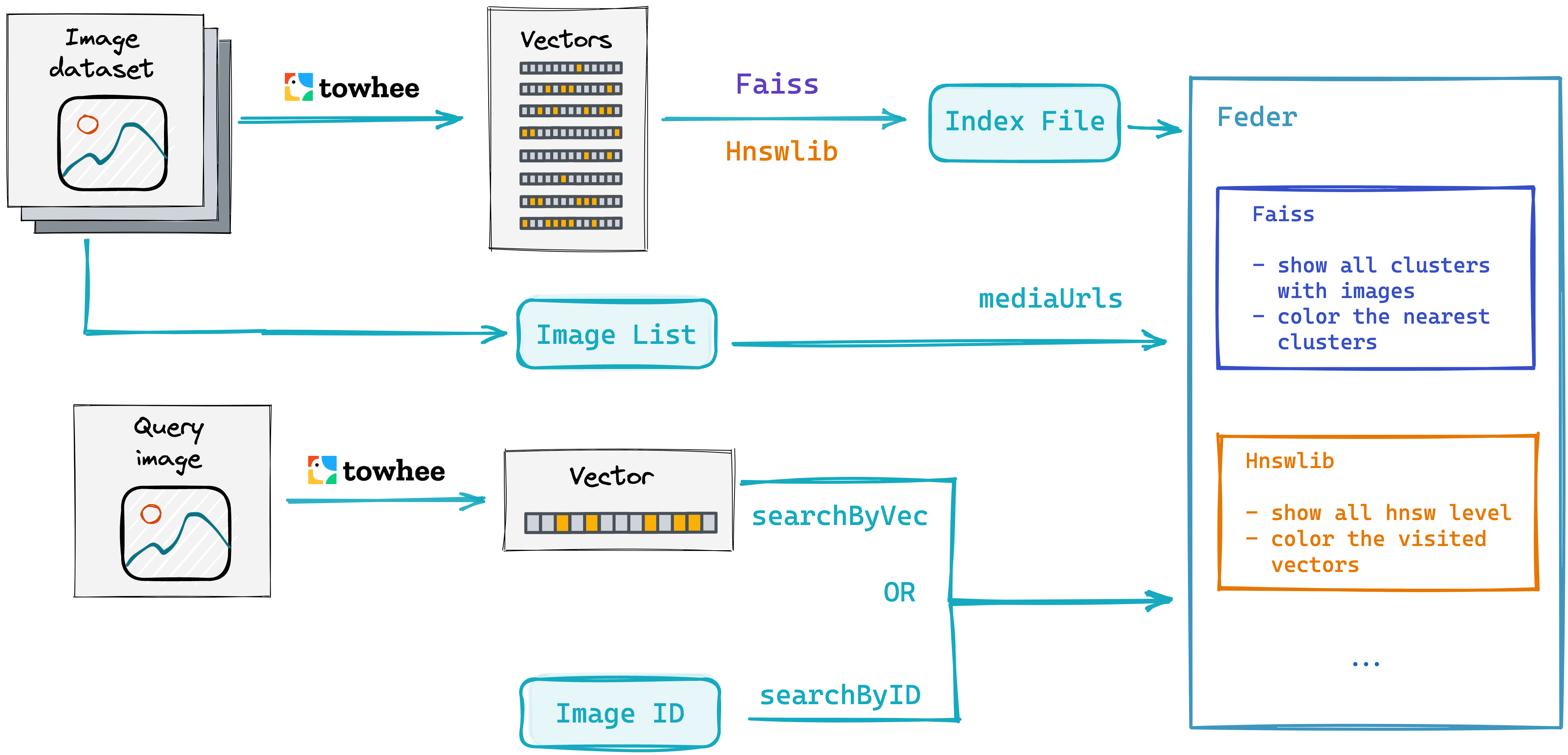
The process of visualize reverse image search is mainly divided into three steps:
- First generate feature vector of the image dataset, and get image list for Feder to show images by
mediaUrls. - Insert the vector into FAISS/HNSWLib, then create the index and save the index file.
- Feder reads the index file and visualizes the process of searching for images. And Feder support
searchByIDorSearchByVecfor the quey image.
- Install dependencies
First to install the related dependencies, such as feder, towhee, hnswlib and numpy.
Please install faiss with conda in your env, such asconda install -c pytorch faiss-cpu, or you can try pip install faiss-cpu(not official).
$ python -m pip -q install federpy towhee hnswlib numpy
- Prepare the data
Then to download the image dataset, which is a subset of the ImageNet dataset (100 classes, 10 images for each class) and it is available via Github.
$ curl -L https://github.com/towhee-io/examples/releases/download/data/reverse_image_search.zip -O
$ unzip -q -o reverse_image_search.zip
This imageset is the same data in "Build a Milvus Powered Image Search Engine in Minutes" and "Deep Dive into Real-World Image Search Engine with Towhee" notebook. Next to get all images in the train directory, images will be used for Feder to display data.
import towhee

images = towhee.glob('train/*/*.JPEG').to_list()
- Generate Image Feature Vector
We use image_embedding.timm operator to generate image vectors, this operator is form Towhee hub and it supports a variety of image models, including vgg16, resnet50, vit_base_patch8_224, convnext_base, etc.
import numpy as np

dc = (towhee.glob('train/*/*.JPEG')
          .image_decode()
          .image_embedding.timm(model_name='resnet50')
          .to_list()
     )

vectors = np.array(dc, dtype="float32")
- Train and add data to Faiss
The save_faiss_index function is defined here to insert the vector data into Faiss and save an index (IVF_FLAT) file. Before adding to faiss, these 1000 pieces of data are also used for training, and the IVF_FLAT index parameter is nlist=128.
import faiss

def save_faiss_index(vec, file_name):
    dim = vec.shape[1]
    nlist = 128
    faiss_index = faiss.index_factory(dim, 'IVF%s,Flat' % nlist)
    faiss_index.train(vec)
    faiss_index.add(vec)

    faiss.write_index(faiss_index, file_name)

save_faiss_index(vectors, 'faiss.index')
- Add data to HNSWLib and create index
Similarly, the save_hnswlib_index function here is used to insert the vector into HNSWLib and save the index (HNSW) file, where the index parameters are ef_construction=30, M=6.
import hnswlib

def save_hnsw_index(vec, file_name):
    dim = vec.shape[1]
    max_elements = vec.shape[0]
    hnsw_index = hnswlib.Index(space='l2', dim=dim)
    hnsw_index.init_index(max_elements=max_elements, ef_construction=30, M=6)
    hnsw_index.add_items(vec)

    hnsw_index.save_index(file_name)

save_hnsw_index(vectors, 'hnswlib.index')
- Search in Faiss and visualization
Next to define the get_faiss_feder function, which uses Feder to read the index file from Faiss, the mediatType is set to img, and the mediaUrls is images. The images is declare before, which is used to display all images in Feder. In addition, the search parameters of faiss are k=5, nprobe=6.
from federpy.federpy import FederPy

def get_faiss_feder(faiss_index_file_name):
    viewParams = {
        "width": 950,
        "height": 600,
        "mediaType": "img",
        "mediaUrls": images,
        "fineSearchWithProjection": 1,
        "projectMethod": "umap"
    }
    faiss_feder = FederPy(faiss_index_file_name, 'faiss', **viewParams)
    faiss_feder.setSearchParams({"k": 5, "nprobe": 6})
    return faiss_feder
Before search vector with Feder, let's take a look about Faiss' IVF_FLAT index:
- The feature space is partitioned into nlist cells.
- The database vectors are assigned to one of these cells thanks using a quantization function (in the case of k-means, the assignment to the centroid closest to the query), and stored in an inverted file structure formed of nlist inverted lists.
- At query time, a set of nprobe inverted lists is selected
- The query is compared to each of the database vector assigned to these lists.
Next, we can get the faiss feder and visualize the index. Below is an example of retrieving a picture with id 40, you can see the basic information of the index (1000 vectors, divided into 128 clusters) and the process of retrieving the information (finding the 6 closest clusters) are listed on the left. And there are three options of "Coarse Search", "Fine Search (Distance)" and "Fine Search (Project)", you can choose to change the style of the board.
The entire board is divided into 128 (nlist=128) clusters, each cluster displays the corresponding pictures (9 pictures in the cluster are randomly displayed), and the highlighted part is the 6 (nprobe=6) clusters closest to the query picture during the retrieval process, the circle is the cluster center point closest to the query image.
faiss_feder = get_faiss_feder('faiss.index')
faiss_feder.searchById(40)
- Search in HNSWLib and visualization
Similar to Faiss, we first define the get_hnsw_feder function to read the index file from hnswlib, where the mediaType is img, the mediaUrls here is the images declared earlier, and the query parameters of HNSW index is k=5, ef_search=6.
from federpy.federpy import FederPy

def get_hnsw_feder(hnsw_index_file_name):
    viewParams = {
        "width": 950,
        "height": 600,
        "mediaType": "img",
        "mediaUrls": images,
    }
    hnsw_federPy = FederPy(hnsw_index_file_name, 'hnswlib', **viewParams)
    hnsw_federPy.setSearchParams({"k": 5, "ef_search": 6})
    return hnsw_federPy
Before search vector with Feder, let's learn about HNSW (Hierarchical Navigable Small World Graph) index, which is a graph-based indexing algorithm. It builds a multi-layer navigation structure for an image according to certain rules. In this structure, the upper layers are more sparse and the distances between nodes are farther; the lower layers are denser and the distances between nodes are closer. The search starts from the uppermost layer, finds the node closest to the target in this layer, and then enters the next layer to begin another search. After multiple iterations, it can quickly approach the target position.
Next, we can get hnsw feder and visualize the index. Here is an example of retrieving a image with an id of 40. You can see that the basic information of the index (1000 vectors, including 4 levels) and the information of the process of retrieval vector (130 of these vectors were visited in total) is listed on the left.
The entire board shows 4 layers and the retrieval process for each layer. First, find the nearest vectors in the first three layers (Level 3, 2, 1), whihc is colored with red dots. Then 111 vectors are visited in the last layer, and the nearest vector is find. The five results closest to the query vector are indicated by red dots at the Level 0 layer.
hnsw_federPy = get_hnsw_feder('hnswlib.index')
hnsw_federPy.searchById(40)
In the previous codelab("Build a Milvus Powered Image Search Engine in Minutes") we found that normalizing the vector can improve the accuracy of the reverse image search, so let's take a look about the retrieving process with normalized vectors.
First we extract the feature vector of the image and then normalize the vector.
dc_norm = (towhee.glob('train/*/*.JPEG')
          .image_decode()
          .image_embedding.timm(model_name='resnet50')
          .tensor_normalize()
          .to_list()
          )

vectors_norm = np.array(dc_norm, dtype="float32")
Next insert the normalized vector into Faiss and Hnswlib, then return the corresponding index file.
save_faiss_index(vectors_norm , 'faiss_norm.index')
save_hnsw_index(vectors_norm , 'hnswlib_norm.index')
WARNING clustering 1000 points to 128 centroids: please provide at least 4992 training points
There is the Faiss index after normalization:
faiss_feder_norm = get_faiss_feder('faiss_norm.index')
faiss_feder_norm.searchById(40)
There is the HNSW index after normalization:
hnsw_federPy_norm = get_hnsw_feder('hnswlib_norm.index')
hnsw_federPy_norm.searchById(40)
In the previous codelab ("Deep Dive into Real-World Image Search Engine with Towhee"), we know that object detection performs well when retrieving partial data, next we compare the retrieval process with and without object detection.
The get_object function is used to get the image of the object detected by YoLov5, or the image itself if there is no object. First, we can get the feature vector of the same image after detecting object, as well as the feature vector of the original image.
def get_object(img, boxes):
    if len(boxes) == 0:
        return img
    max_area = 0
    for box in boxes:
        x1, y1, x2, y2 = box
        area = (x2-x1)*(y2-y1)
        if area > max_area:
            max_area = area
            max_img = img[y1:y2,x1:x2,:]
    return max_img

images_obj = towhee.glob('./object/*.jpg').to_list()

dc_img = (towhee.glob['path']('./object/*.jpg')
          .image_decode['path', 'img']()
          .image_embedding.timm['img', 'vec'](model_name='resnet50')
          .tensor_normalize['vec', 'vec']()
          .select['vec']()
          .as_raw()
          .to_list()
     )

dc_obj = (towhee.glob['path']('./object/*.jpg')
          .image_decode['path', 'img']()
          .object_detection.yolov5['img', ('boxes', 'class', 'score')]()
          .runas_op[('img', 'boxes'), 'object'](func=get_object)
          .image_embedding.timm['object', 'object_vec'](model_name='resnet50')
          .tensor_normalize['object_vec', 'object_vec']()
          .select['object_vec']()
          .as_raw()
          .to_list()
     )

vectors_img = np.array(dc_img, dtype="float32")
vectors_obj = np.array(dc_obj, dtype="float32")
We first retrieve the original image vector (without object detection), we can see that the closest clusters to the original image are various strange images, and there are 17 various images in the cluster 69 where the nearest center point is located. Then we can click Fine Search, we can see the 5 results about spider, it's same as the "Deep Dive into Image Search" code lab.
faiss_feder_norm = get_faiss_feder('faiss_norm.index')
faiss_feder_norm.searchByVec(vectors_img[0], images_obj[0]) #Search without object detection
The vectors with object detection are all images of cars in the nearest cluster0.
faiss_feder_norm = get_faiss_feder('faiss_norm.index')
faiss_feder_norm.searchByVec(vectors_obj[0], images_obj[0]) #Search with object detection
The visualization of cross-modal search is the last and most interesting, it uses towhee clip Operator to extract feature vectors of images and text, if the content of the image and text description are similar, their vector distances will also be very close.
First, we use cilp to generate feature vectors for all images, and we need to set modality='image'.
dc_img = (towhee.glob('train/*/*.JPEG')
          .image_decode()
          .towhee.clip(model_name='clip_vit_b32', modality='image')
          .tensor_normalize()
          .to_list()
          )

vectors_img = np.array(dc_img, dtype="float32")
Insert all image vectors into Hnswlib and return the index file.
save_hnsw_index(vectors_img, 'hnswlib_cm.index')
Next, we will search for images using text, first generating a vector of text and then using searchByVec to search in Feder. We can use the Cilp operator to get the feature vector of ‘A white dog' and "a black dog" by setting modality=‘text'.
dc_text = (towhee.dc(['A white dog.', 'A black dog'])
            .towhee.clip(model_name='clip_vit_b32', modality='text')
            .tensor_normalize()
            .to_list()
           )
vectors_text = np.array(dc_text, dtype="float32")
To search ‘A white dog' in Hnswlib, the retrieval process is as follows:
hnsw_federPy_cm = get_hnsw_feder('hnswlib_cm.index')
hnsw_federPy_cm.searchByVec(vectors_text[0]) #search the white dog
Search for ‘A Black dog' in Hnswlib as follows, you can see that although the results are all pictures of dogs, the retrieval process is quite different.
When retrieving white dogs, 147 vectors were visited in the last layer, and images of white elements were found in the second layer(Level 2). When retrieving black dogs, 89 vectors were visited in the last layer, and images with black elements were found in the second layer.
hnsw_federPy_cm = get_hnsw_feder('hnswlib_cm.index')
hnsw_federPy_cm.searchByVec(vectors_text[1]) #search the black dog